Naive Bayes classifier

Table of Contents

Naive Bayes Classifier Algorithm

The Naive Bayes classifier is a probabilistic algorithm that is based on Bayes’ theorem. It is called “naive” because it assumes independence between the features, which is rarely the case in real-world data. Despite this assumption, it often performs well in practice and is particularly useful for high-dimensional data sets. The algorithm is typically trained using labeled data, where each example is a tuple of features and a label. Once trained, the algorithm can be used to predict the label of new examples based on their features. There are several variations of the algorithm, including the Gaussian Naive Bayes, Multinomial Naive Bayes, and Bernoulli Naive Bayes. It is commonly used in text classification and spam filtering.

In addition to text classification and spam filtering, the Naive Bayes classifier is also commonly used in other applications such as sentiment analysis, medical diagnosis, and weather forecasting.

Why is it called Naïve Bayes?

The Naive Bayes classifier is called “naive” because it makes the strong assumption that all the features in the data are independent of each other. This assumption is often not true in real-world data, as features can be correlated or dependent on each other in various ways. The reason why the algorithm is called “Naive” is because the independence assumption is not realistic and the algorithm is not able to model the complexity of real-world data.

Despite this unrealistic assumption, the Naive Bayes classifier is still widely used and often performs well in practice. This is because the algorithm can still provide good results even if the independence assumption is not entirely true, especially when the number of features is large.

So, the name “Naive Bayes” is used to reflect the naive assumption of independence between features, and to emphasize that the algorithm is based on Bayes’ theorem.

Bayes’ Theorem:

Bayes’ theorem is a fundamental result in probability theory that describes the relationship between the probability of an event occurring (the prior probability), and the probability of the event occurring given some additional information (the posterior probability). It is named after Reverend Thomas Bayes, an 18th-century statistician and theologian who first published the result in his 1763 paper “An Essay towards solving a Problem in the Doctrine of Chances”.

The theorem is stated mathematically as:

P(A|B) = P(B|A) * P(A) / P(B)

where:

P(A|B) is the posterior probability of event A occurring given that event B has occurred
P(B|A) is the likelihood of event B occurring given that event A has occurred
P(A) is the prior probability of event A occurring
P(B) is the prior probability of event B occurring.

This theorem is used in many areas of artificial intelligence and machine learning, including in the Naive Bayes classifier algorithm. It allows the algorithm to use previous knowledge or data to update the probability of an event occurring, given new information.

Working of Naïve Bayes’ Classifier:

The Naive Bayes classifier algorithm uses Bayes’ theorem to classify new data points based on the probability of a certain class given the feature values of the data point. The basic idea is to calculate the probability of each class for a given data point and then select the class with the highest probability as the prediction.

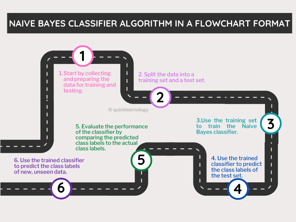
The algorithm works in the following steps:

Collect and preprocess the training data: The training data is a set of labeled examples, where each example is a tuple of feature values and a class label. The data is typically preprocessed to handle missing values, scale the features, and remove any irrelevant features.
Estimate the likelihoods: The algorithm estimates the likelihoods of the feature values for each class by counting the number of occurrences of each feature value in the training data for each class.
Estimate the class priors: The class priors are the probabilities of each class in the training data. These are calculated by counting the number of occurrences of each class in the training data.
Classify new data points: To classify a new data point, the algorithm calculates the probability of each class for the data point by multiplying the class prior by the likelihoods of the feature values for that class. The class with the highest probability is selected as the prediction.
Validate the model: The model is validated using a set of test data to evaluate the accuracy of the predictions.

It’s important to notice that the independence assumption of the features, is used to simplify the calculations, reducing the computational cost.

Advantages of Naïve Bayes Classifier:

The Naive Bayes classifier is a simple and popular algorithm that has several advantages, including:

Computational efficiency: The algorithm is relatively simple and requires relatively little training data, making it computationally efficient. It also scales well to large numbers of features, making it suitable for high-dimensional data.
Handling missing data: The algorithm is able to handle missing data by using the maximum likelihood estimation method, which estimates the likelihoods from the available data.
Robustness to irrelevant features: The algorithm is relatively robust to irrelevant features, as it only considers the relative frequencies of feature values in the training data and not the actual values.
Multi-class classification: The algorithm can easily be extended to handle multi-class classification problems, where the goal is to predict one of several possible classes.
Good performance: Despite the Naive assumption, the Naive Bayes classifier often performs well in practice, especially when the number of features is large.
Easy to interpret: The predictions of the algorithm are easy to interpret, as they are based on the estimated probability of each class.
Fast to train and test: The algorithm is fast to train and test. Even for large data sets, the training and testing time is usually less than other algorithms.
Can be used as a Baseline: Due to its simple nature and good performance, Naive Bayes can often be used as a baseline model to compare the performance of more complex algorithms.

Disadvantages of Naïve Bayes Classifier:

Despite its many advantages, the Naive Bayes classifier also has some disadvantages:

Independence assumption: The most important disadvantage of the Naive Bayes classifier is the assumption that all the features are independent of each other. This assumption is often not true in real-world data, which can lead to poor performance.
Zero probabilities: The algorithm can produce zero probabilities when a feature value has not been seen in the training data. This can be mitigated by using smoothing techniques to add a small value to the likelihoods.
Limited representation: The algorithm can only represent the probability distribution of the data, and it is not able to represent complex relationships between features.
Sensitive to irrelevant features: The algorithm is sensitive to irrelevant features, as they can bias the probability estimates.
Overfitting: The algorithm can overfit the training data when the number of features is large.
Not suitable for continuous features: Naive Bayes is not suitable for continuous features, it only works well with discrete features.
Not suitable for small datasets: The algorithm may not perform well with small datasets as it needs a relatively large number of data points to make accurate predictions.
Not suitable for non-linear problems: Naive Bayes is not suitable for non-linear problems, it only works well with linear problems.

Applications of Naïve Bayes Classifier:

The Naive Bayes classifier algorithm is widely used in various applications, some of the most common include:

Text classification: The algorithm is commonly used for text classification tasks, such as spam detection, sentiment analysis, and topic classification.
Image classification: The algorithm can also be used for image classification tasks, such as object detection and face recognition.
Medical diagnosis: The algorithm has been used in medical diagnosis to predict the presence of a disease based on symptoms and other patient-specific data.
Natural Language Processing (NLP): Naive Bayes is used in many NLP tasks like text classification, sentiment analysis, spam detection, and language detection.
Spam Filtering: The algorithm is used to filter out unwanted emails, by identifying and marking them as spam.
Document classification: The algorithm is used to classify documents based on their content, for example, classifying news articles into different categories like sports, politics, science, etc.
Recommender Systems: The algorithm can also be used in recommendation systems to predict the likelihood that a user will like a particular item based on their past behavior and preferences.
Fraud Detection: Naive Bayes can be used to detect fraudulent activities in financial transactions, by identifying patterns and anomalies in the data.
Weather prediction: Naive Bayes can be used to predict the weather based on historical data, by identifying patterns and trends in the data.

Types of Naïve Bayes Model:

There are several types of Naive Bayes models, including:

Gaussian Naive Bayes: This model is used when the features are continuous and follow a normal distribution. It is often used in applications such as medical diagnosis and image classification.
Multinomial Naive Bayes: This model is used when the features are discrete and represent the frequency of occurrence of a feature. It is often used in applications such as text classification and document classification.
Bernoulli Naive Bayes: This model is also used when the features are discrete and represent binary values (i.e., either 0 or 1). It is used in applications such as spam filtering, where the features represent the presence or absence of specific words in an email.
Complement Naive Bayes: This model is an extension of the Multinomial Naive Bayes, it is used when the data is imbalanced.
Averaged Perceptron Naive Bayes: This model is an extension of the Multinomial Naive Bayes, it is used when there are many irrelevant features.
Neural Network Naive Bayes: This model is an extension of the Naive Bayes algorithm by incorporating a neural network to make predictions.
Decision Tree Naive Bayes: This model is an extension of the Naive Bayes algorithm by incorporating a decision tree to make predictions.
Random Forest Naive Bayes: This model is an extension of the Naive Bayes algorithm by incorporating a random forest to make predictions.

# Assigning features and label variables
weather=['Sunny','Sunny','Overcast','Rainy','Rainy','Rainy','Overcast','Sunny','Sunny',
'Rainy','Sunny','Overcast','Overcast','Rainy']
temp=['Hot','Hot','Hot','Mild','Cool','Cool','Cool','Mild','Cool','Mild','Mild','Mild','Hot','Mild']
play=['No','No','Yes','Yes','Yes','No','Yes','No','Yes','Yes','Yes','Yes','Yes','No']



# Import LabelEncoder
from sklearn import preprocessing


#creating labelEncoder
le = preprocessing.LabelEncoder()


# Converting string labels into numbers.
weather_encoded=le.fit_transform(weather)
print (weather_encoded)


# Converting string labels into numbers
temp_encoded=le.fit_transform(temp)
label=le.fit_transform(play)
print ("Temp:",temp_encoded)
print ("Play:",label)


#Combinig weather and temp into single listof tuples
features=zip(weather_encoded,temp_encoded)
features= list(features)
print (features)


#Import Gaussian Naive Bayes model
from sklearn.naive_bayes import GaussianNB


#Create a Gaussian Classifier
model = GaussianNB()


# Train the model using the training sets
model.fit(features,label)


#Predict Output
predicted= model.predict([[0,2]]) # 0:Overcast, 2:Mild
print ("Predicted Value:", predicted)


#Import scikit-learn dataset library
from sklearn import datasets
#Load dataset
wine = datasets.load_wine()


# print the names of the 13 features
print ("Features: ", wine.feature_names)


# print the label type of wine(class_0, class_1, class_2)
print ("Labels: ", wine.target_names)


# print data(feature)shape
wine.data.shape


# print the wine data features (top 5 records)
print (wine.data[0:5])


# print the wine labels (0:Class_0, 1:class_2, 2:class_2)
print (wine.target)


# Import train_test_split function
#from sklearn.cross_validation import train_test_split
from sklearn.model_selection import train_test_split


# Split dataset into training set and test set
X_train, X_test, y_train, y_test = train_test_split(wine.data, wine.target, test_size=0.3,random_state=109) # 70% training and 30% test


!pip install scikit-learn


# Import train_test_split function
from sklearn.model_selection import train_test_split


# Split dataset into training set and test set
X_train, X_test, y_train, y_test = train_test_split(wine.data, wine.target, test_size=0.3,random_state=109) # 70% training and 30% test


#Import Gaussian Naive Bayes model
from sklearn.naive_bayes import GaussianNB


#Create a Gaussian Classifier
gnb = GaussianNB()


#Train the model using the training sets
gnb.fit(X_train, y_train)


#Predict the response for test dataset
y_pred = gnb.predict(X_test)


#Import scikit-learn metrics module for accuracy calculation
from sklearn import metrics


# Model Accuracy, how often is the classifier correct?
print("Accuracy:",metrics.accuracy_score(y_test, y_pred))