Rosenblatts Perceptron

The Perceptron algorithm is a type of neural network that was introduced by Frank Rosenblatt in 1958. It is a basic algorithm that uses a single-layer neural network to classify data into two classes. The Perceptron algorithm is still widely used today, and it has been shown to be effective in a variety of applications.

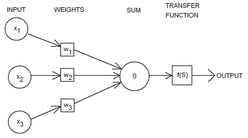
One of the key advantages of the Perceptron algorithm is that it is simple to understand and implement. It uses a single-layer neural network with a linear activation function to classify data. The algorithm works by iteratively adjusting the weights of the inputs to the neural network until the desired classification accuracy is achieved.

One of the challenges with the Perceptron algorithm is that it is only effective for linearly separable data. This means that the data can be separated into two categories using a straight line. If the data is not linearly separable, the Perceptron algorithm may not be able to achieve high classification accuracy.

Despite this limitation, the Perceptron algorithm remains a popular choice for many machine learning applications. It is particularly useful for problems that involve binary classification, where it can be used to quickly and efficiently classify data into two categories.

In conclusion, the Perceptron algorithm is a simple yet powerful algorithm that can be used for a variety of machine learning applications. It is particularly useful for problems that involve binary classification, and it remains a popular choice for many researchers and practitioners in the field of machine learning.

from sklearn import datasets
import matplotlib.pyplot as plt
X,y = datasets.make_blobs(n_samples=150,n_features=2,
                         centers=2,cluster_std=1.05,
                         random_state=2)

#Plotting
fig = plt.figure(figsize=(10,8))
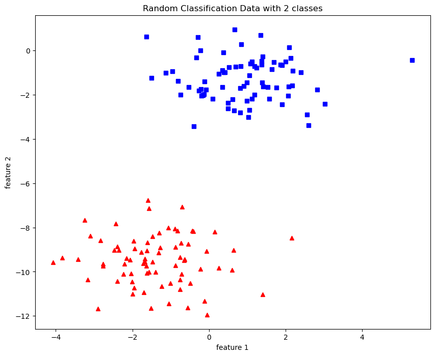
plt.plot(X[:,0][y==0],X[:,1][y==0],'r^')
plt.plot(X[:,0][y==1],X[:,1][y==1],'bs')
plt.xlabel("feature 1")
plt.ylabel("feature 2")
plt.title('Random Classification Data with 2 classes')

O/P : Text(0.5, 1.0, ‘Random Classification Data with 2 classes’)

def step_func(z):
    return 1.0 if(z > 0) else 0.0

import numpy as np
def perceptron(X, y, lr, epochs):

  #X --> Inputs
  #y --> labels/target
  #lr --> learning rate.
  # epochs --> number of iterations.

  # m --> no. of training examples
  # n --> no. of features

    m,n = X.shape

  # initializing parapeter(theta) to zeros.
  # +1 in n+1 for the bias term.
    theta = np.zeros((n+1,1))

  # Empty list to store how many examples were
  # misclassified at every iteration.
    n_miss_list = []

  #Training.
    for epoch in range(epochs):

    # variable to store 
    #misclassified.
        n_miss = 0
    # looping for every example.
        for idx, x_i in enumerate(X):

      #Inserting 1 for bias, X0 = 1
            x_i =  np.insert(x_i, 0, 1).reshape(-1,1)

       # Claculating prediction/hypothesis
            y_hat = step_func(np.dot(x_i.T, theta))

       #Updating if the example is misc;lassified.
            if(np.squeeze(y_hat) - y[idx]) != 0:
                  theta += lr*((y[idx] - y_hat)*x_i)

         #Incrementing by 1.
            n_miss += 1

         #Appending no. of misclassified examples
         # at every iteration
            n_miss_list.append(n_miss)

        return theta, n_miss_list

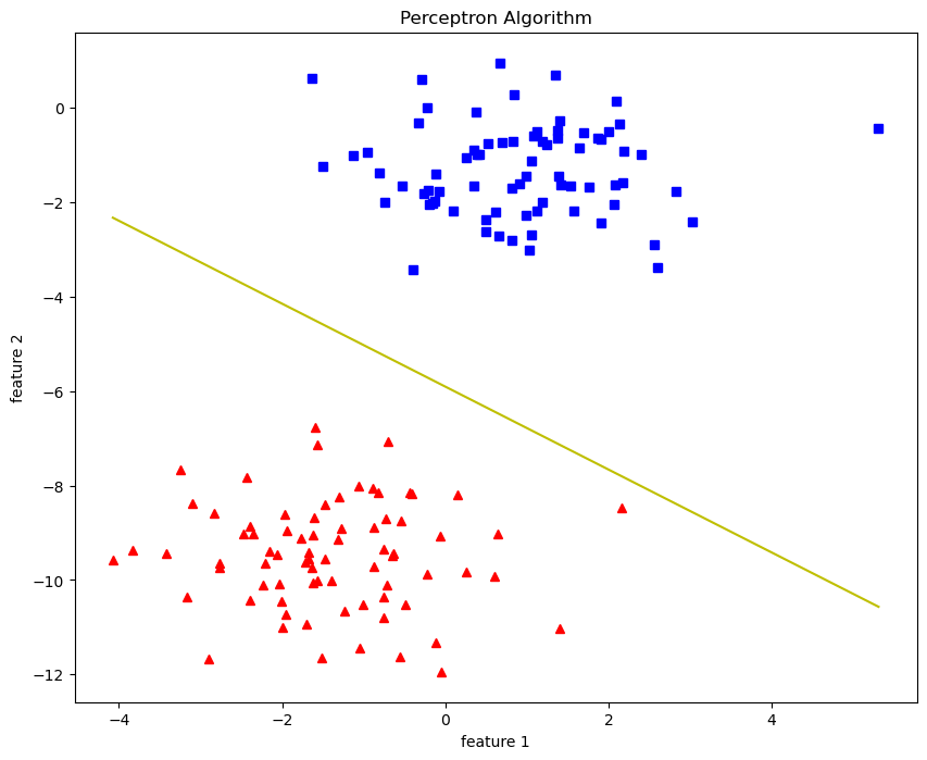
def plot_decision_boundary(x,theta):
    #x --->> Inputs
    #theta --->> parameters
    #the line is y=mx+c
    #So equate mx+c = theta0.X0 + theta1.X1 + theta2.X2
    
    #solving we find m and c
    
    x1 = [min(X[:,0]),max(X[:,0])]
    m = -theta[1]/theta[2]
    c = -theta[0]/theta[2]
    x2 = m*x1 + c

    #Plotting
    fig = plt.figure(figsize=(10,8))
    plt.plot(X[:,0][y==0],X[:,1][y==0],'r^')
    plt.plot(X[:,0][y==1],X[:,1][y==1],'bs')
    plt.xlabel("feature 1")
    plt.ylabel("feature 2")
    plt.title('Perceptron Algorithm')
    plt.plot(x1,x2,'y-')

theta,miss_1 = perceptron(X,y,0.5,100)
plot_decision_boundary(X,theta)